
Determining the number of clusters is one of the research questions attracting considerable interests in recent years. Majority of the existing methods require parametric assumptions and substantiated computations. In this work (paper), we proposed a simple yet powerful method for determining the number of clusters based on curvature. Our technique is computationally efficient and straightforward to implement. We compare our method with 6 other approaches on a wide range of simulated and real-world datasets. Theoretical motivation underlying the proposed method is also presented.
Maxinum Curvature Point at the Evaluation Graph
Evaluation Graph
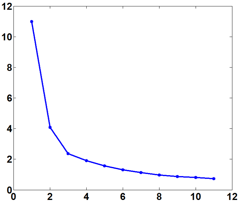
In order to find the appropriate number of clusters, some approaches construct an evaluation graph by taking the x-axis as the cluster number and the y-axis as the corresponding evaluation function value. In these graphs, the within-cluster variance is often used as the evaluation metric.
\[J(k)=\sum\limits_{j=1}^{k}\sum\limits_{x_i\in C_j}||x_i-\overline{x}_j||\]where \(C_j\) is the set of samples belonging to class \(j\) and \(\overline{x}_j\) is the sample mean of class \(j\).
One can then examine the characteristics of such an evaluation graph to determine the number of clusters. A basic idea is to identify the knee or elbow of the evaluation graph.
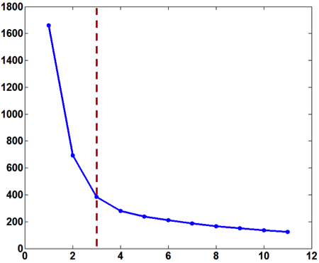
The evaluation graph is monotonically decreasing as the within-cluster variance will decline as the cluster number $k$ increases. However, the decrease in the within-cluster variance would become much smaller when $k$ surpasses the true cluster number, as after this point creating more clusters only lead to partitions within groups rather than between groups. Therefore, one can visually inspect the knee of the evaluation curve which corresponds to the correct number of cluster.
Curvature of Evalutation Graph
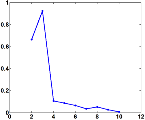
However, determining the knee position of the evaluation curve is actually a non-trivial problem. The visual inspection method is ambiguous especially when there is a high degree of intermix between the clusters. In order to reduce the ambiguity stemming from the process of visual inspection an idea is to use the curvature information of the evaluation graph. In mathematics, curvature is the amount by which a geometric object deviates from being flat, or straight in the case of a line. So the \textit{knee} in the graph should correspond to the point with the maximum curvature. For a curve explicitly given as $y=f(x)$ , the curvature is defined as: \(\kappa=\frac{|y''|}{(1+{y'}^2)^{\frac{3}{2}}}\)
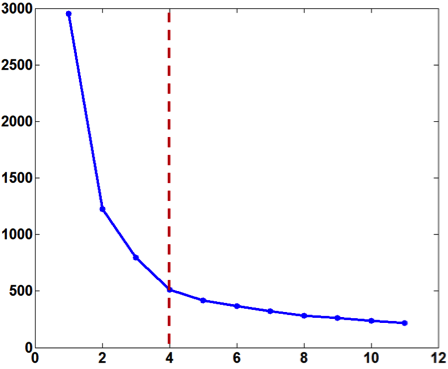
As an example, this curvature method is applied to a real-world dataset (Seed from UCI). The within-cluster variance and the corresponding curvature graph are presented in Figure 2. The true cluster number (equal to 3) corresponds to the maximum curvature point.
Rescale Problem
While computing the curvature, a critical problem was discovered. It was observed that the position of the maximum curvature point changes when the original data is rescaled. Curvature is a kind of geometric property of the graph and tightly related to the range of the two axes. In the evaluation graph, the x-axis is the number of clusters, the difference of which is always one and the y-axis is the within-group variance, the range of which lies in a large variety (often much bigger than the range of x). When the original data is rescaled, the x-axis remains the same and the y-axis has a linear change as indicated below.
\[\kappa_a(k)=\frac{|a^2J''|}{(1+a^4J^{'2})^{\frac{3}{2}}}=\beta(k)\kappa(k)\]where \(\beta(k)=a^2{(\frac{1+a^4J^{'2}}{1+J^{'2}})}^{\frac{3}{2}}\)
For each \(k\), the change of curvature \(\beta (k)\) is not only related to \(a\), but also to \(J^{'}\). This non-linear change in the curvature will cause the shift of the maximum curvature point. As we know, while rescaling the data, the cluster structure in fact remains the same and so does the cluster number. Therefore, although the raw curvature can serve as an effective way to identify the knee of the evaluation graph, it is indeed a poor indicator of cluster number. It should be noted that the traditional knee method suffers from the same scaling problem. When the within-cluster variance against \(k\) is plotted, the software usually automatically scales the range of axes for representation purpose because the range of within-cluster variance is often much bigger than \(k\). When the knee of the graph is inspected visually, it is actually being examined under some scaling factor and thus the results may be unreliable.
Beyond Curvature
Our goal is to eliminate the influence of the scaling factor and at the same time still exploit the usefulness of curvature in the detection of the knee on a graph. To this end a new curvature-based index is proposed which does not depend on the scaling factor.
For convenience, let’s define a scale parameter \(\alpha = a^2\). The curvature of evaluation graph can be expressed as a function with respect to \(k\) and \(\alpha\):
\[\kappa(\alpha,k)=\frac{|\alpha J''(k)|}{(1+\alpha^2{J'(k)}^2)^{\frac{3}{2}}}\]Since the goal is to focus on the influence of \(k\) and to eliminate the effect of $\alpha$, this work proposes to choose the optimal $k$ by solving the following optimization problem.
\[K=\underset{k}{\mathop{\arg\max}}\,\underset{\alpha}{\mathop{\max}}\,\kappa(\alpha,k)\]After some derivations, we have: \(K=\underset{k}{\mathop{\arg\max}}\,|\frac{J''(k)}{J'(k)}|\)
Experiments
The proposed curvature-based method was compared with 6 other well-known approaches of comparable computational complexity: the CH method, the KL method, the Hartigan method, the Silhouette method, the Gap method, the Jump method. The detail descriptions of these six approaches can be found in the original paper.
Prediction Accuracy of Cluster Number
The proposed method outperformed other six approaches on synthetic and real-world datasets. Detail can be found in the paper.
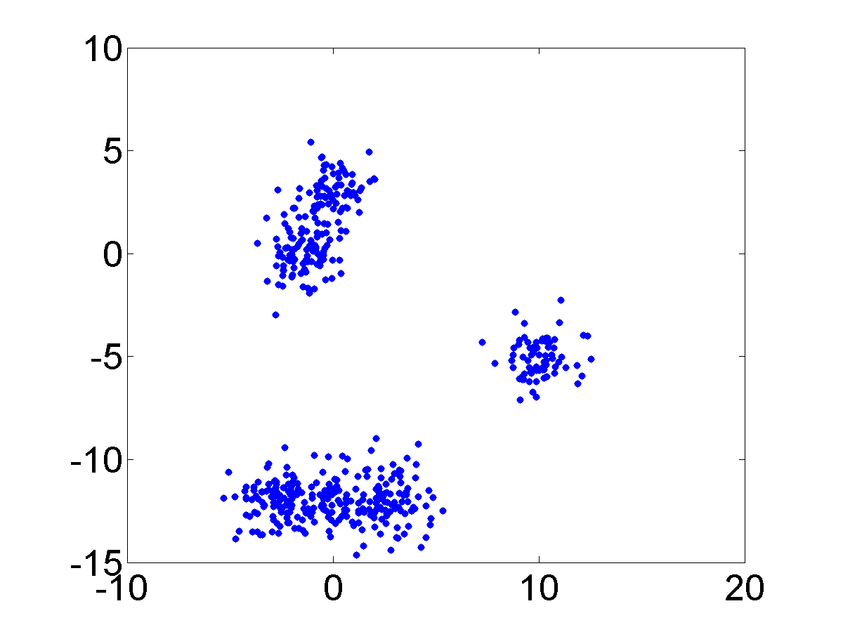
Detection of Hierarchical Cluster Structure
| Datasets | Curvature-based method | Jump method |
|---|---|---|
 |
 |
 |
 |
 |
 |
 |
 |
 |
Compounded Cluster
Dataset
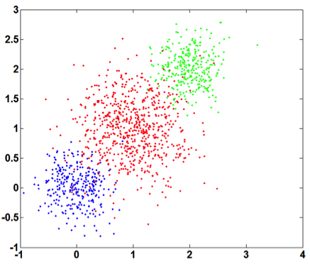
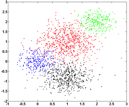
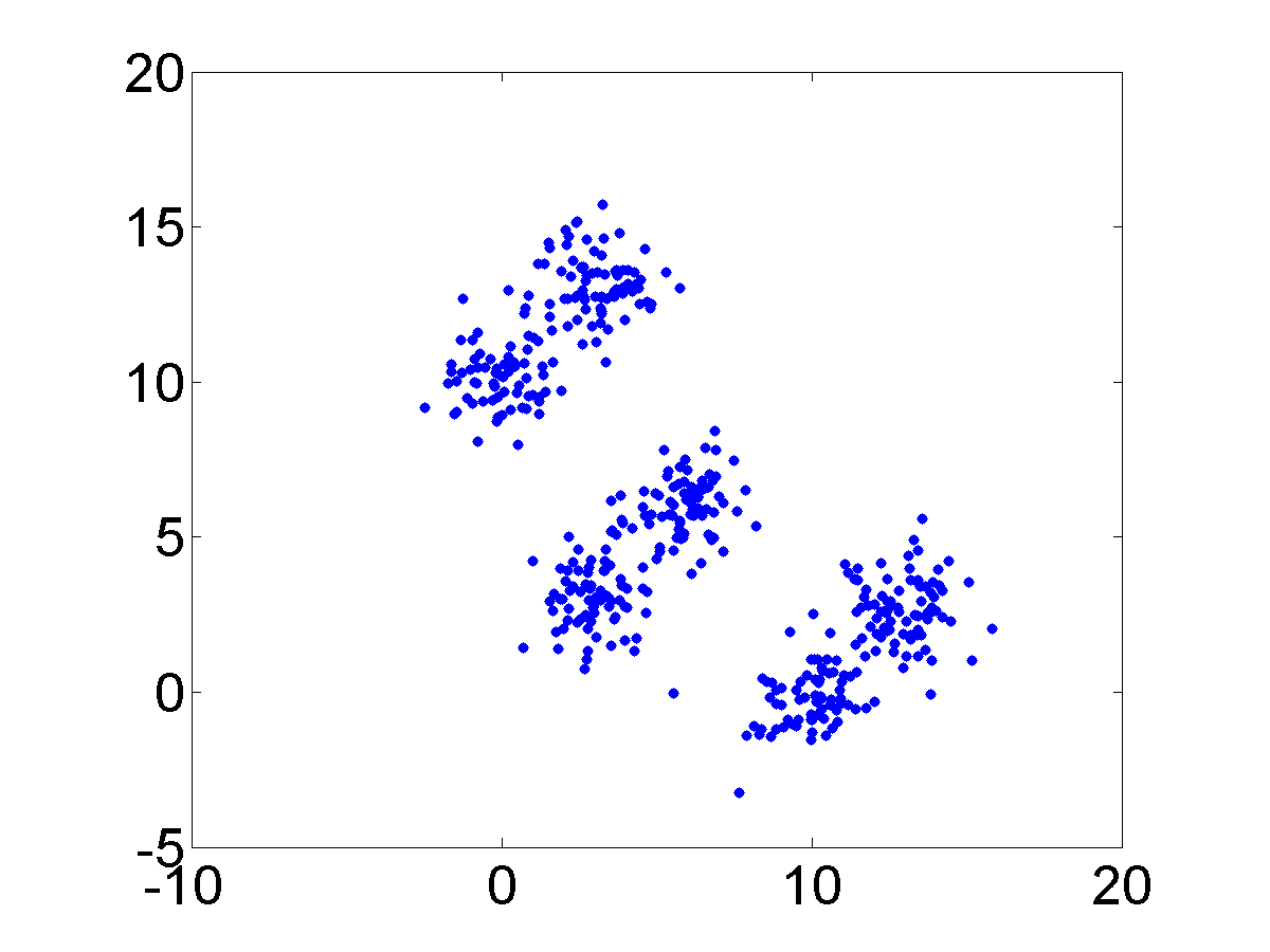
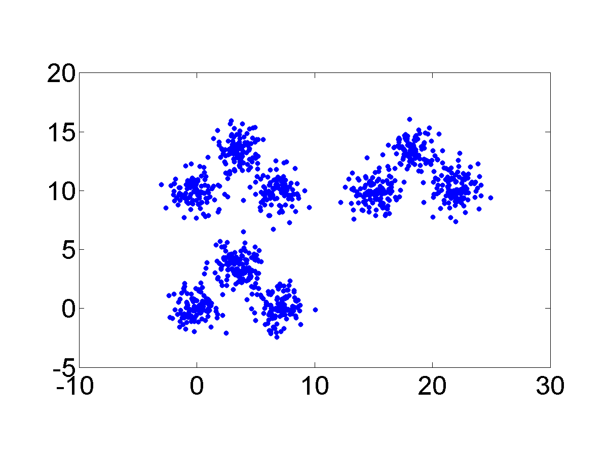
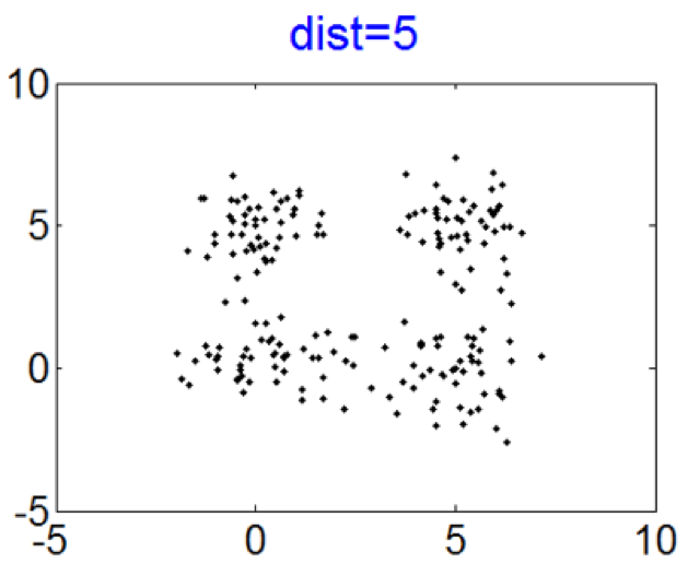
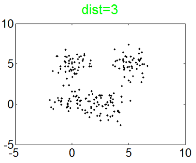
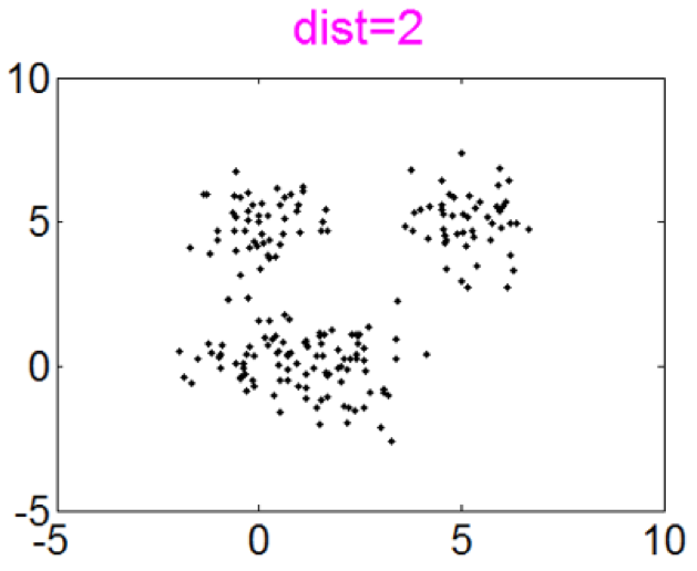
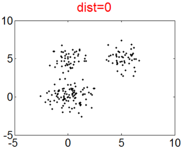
This simulation is designed to investigate how the Curvature index value changes when the extent of intermix between the clusters varies. To this end, four Gaussian clusters in two dimensions which are spaced in a square with the side length of 5 are generated. Each cluster has {a standard \color{black}deviation} of 1 in each dimension. Then the intermix between clusters is introduced by moving one cluster closer to another. More specifically, the distance between two clusters is varied from 5 to 0. Figure 3 presents the datasets with distances equal to 5, 3, 2 and 0. The initial dataset contains 4 clusters and the last one contains 3 clusters. The second and the third ones record the transition from 4 to 3 clusters.
Result
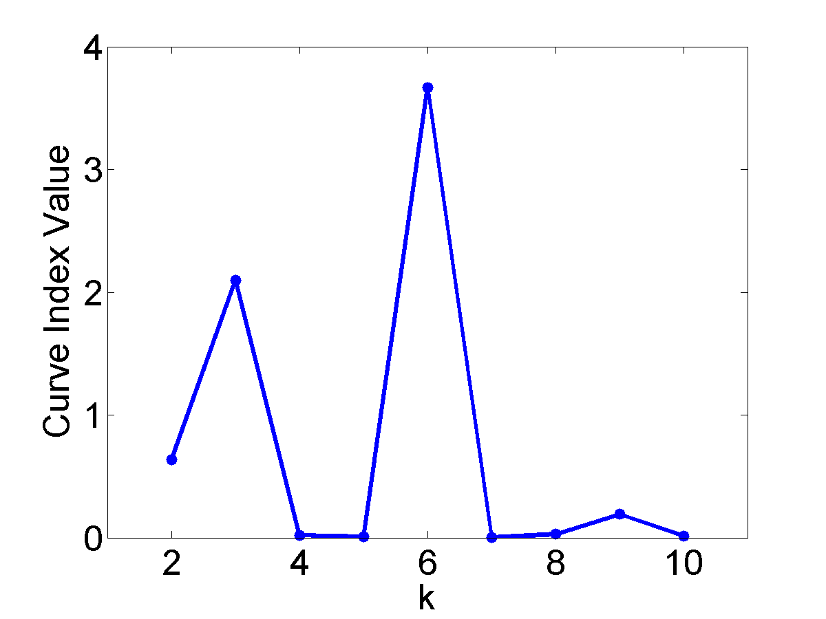
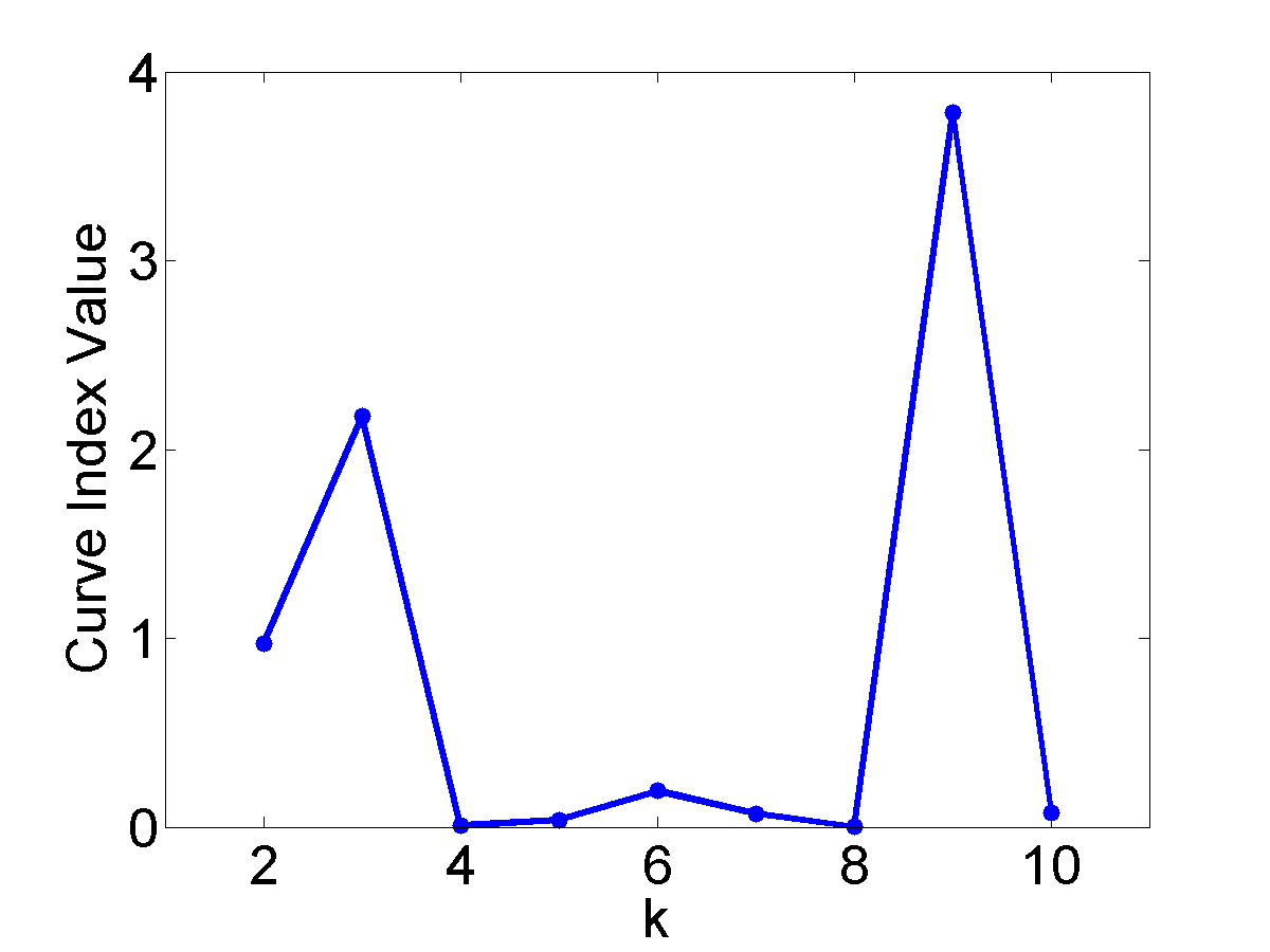
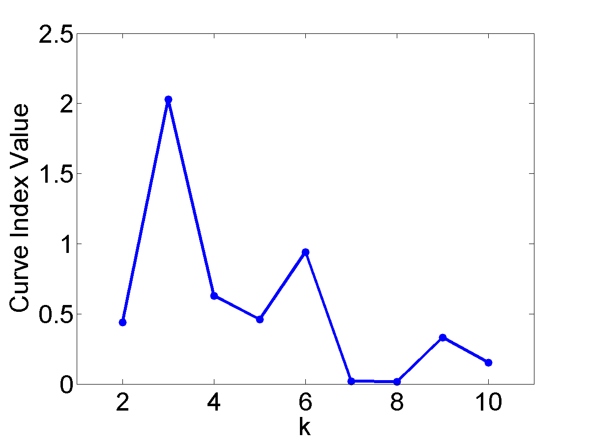
The Curvature index graphs are shown in Figure. The Curvature method estimates the first two datasets as consisting of 4 clusters and the other two as consisting of 3 clusters.
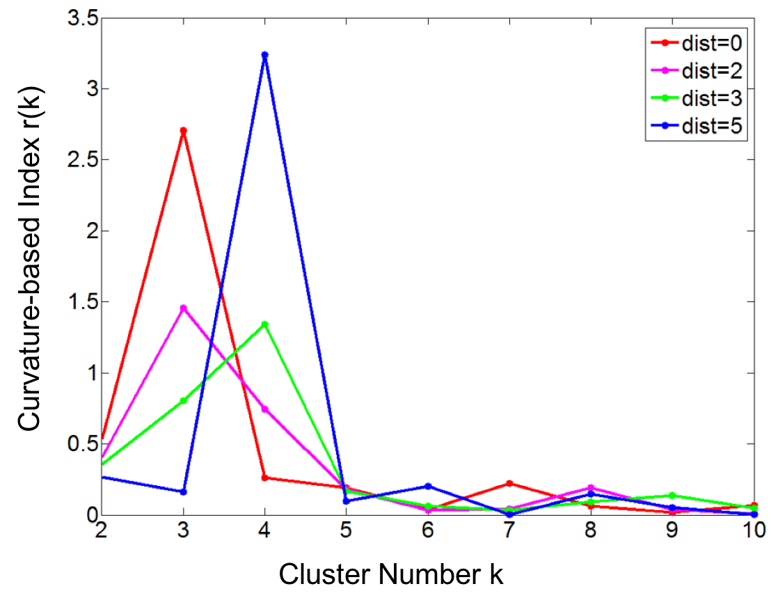
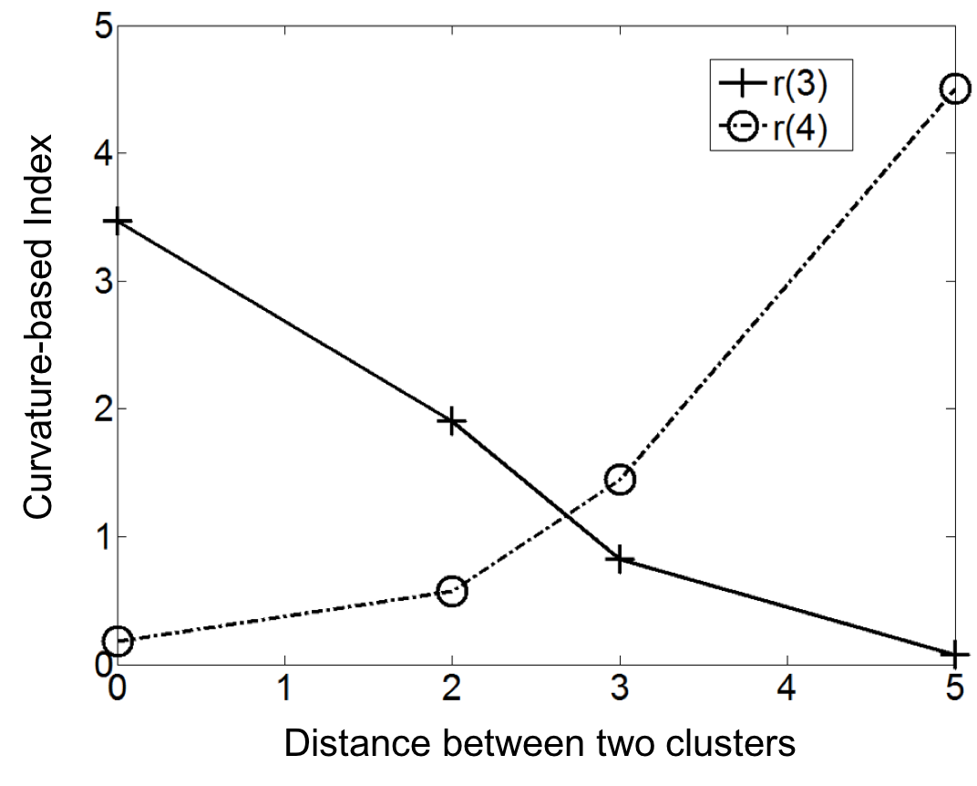
Since the definition of a cluster is not precise, we choose not to judge whether the results are correct or not. Instead we seek to analyze the reasonableness of the Curvature index. Firstly, it can be observed that for all the four datasets the maximum point appears either at \(k=3\) or \(k=4\) and the values for other $k$ are very low, which indicates the low noise level of the proposed Curvature index. Secondly, as the distance between the two clusters increases, the Curvature index at $k=4$ decreases and Curvature index at \(k=3\) increases. This phenomenon corresponds very well to the fact that the data is actually transformed from 4 to 3 clusters. Another interesting observation is that the maximum peaks in the index graph of dataset #1 and #4 are more distinctive than the peaks in dataset #2 and #3. This conforms to the fact that dataset #1 and #4 have clearer cluster structure than the other two datasets.
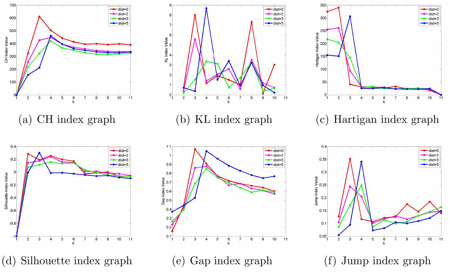
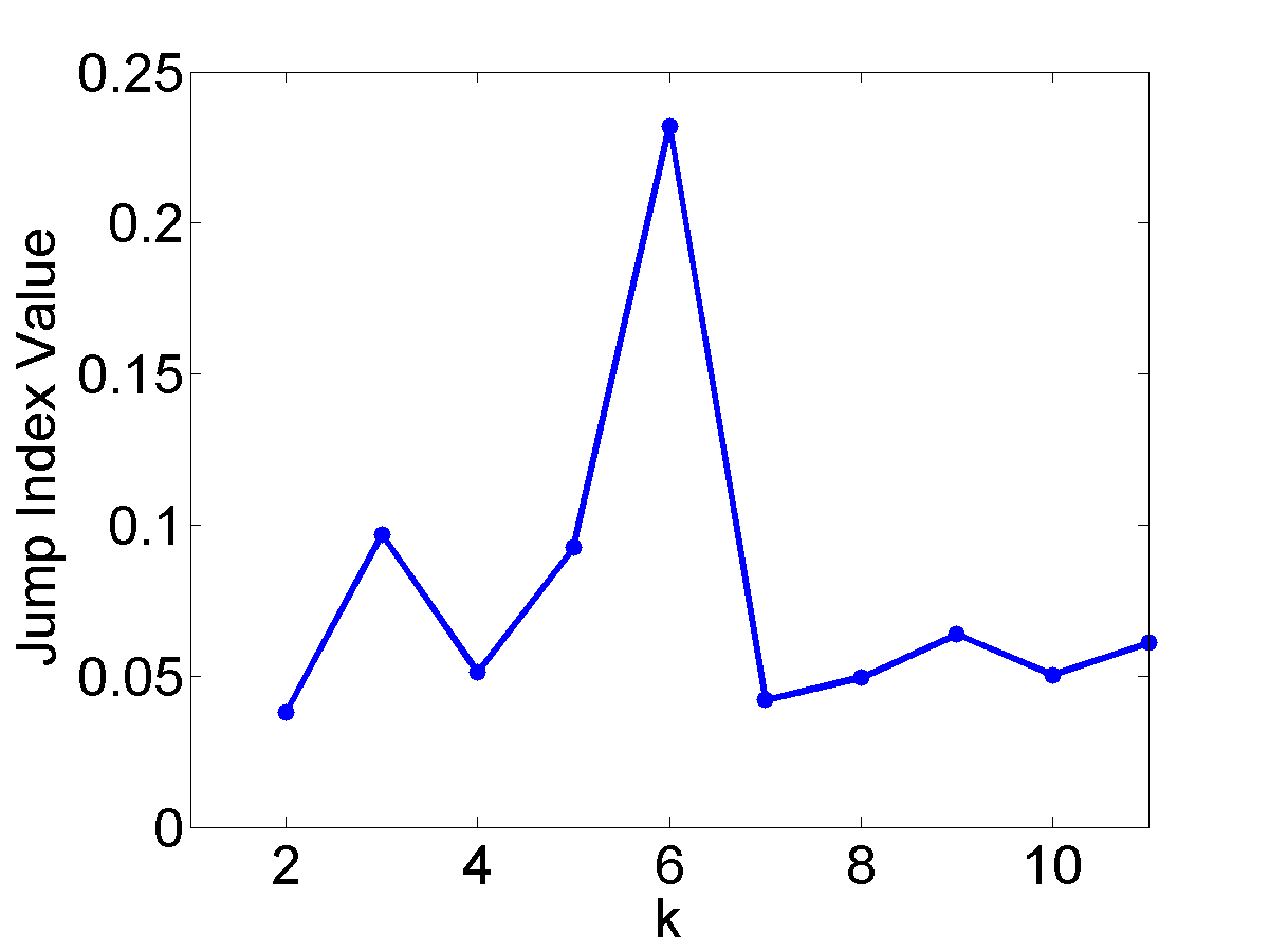
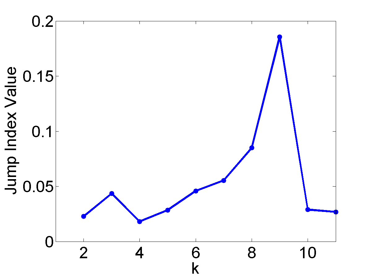
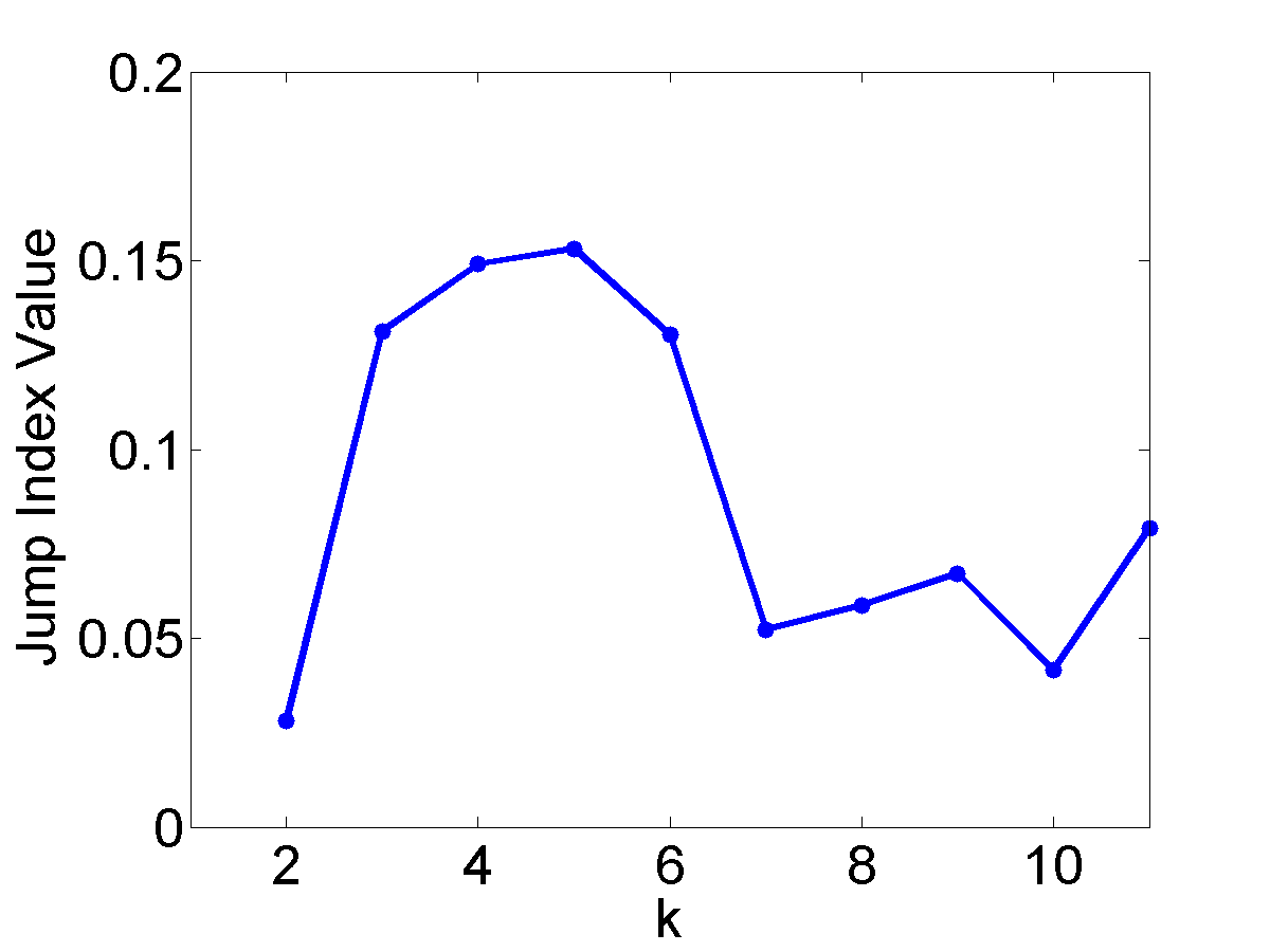
The performance of the 6 existing approaches on the four datasets are shown in Figure 5. It can be seen that the maximum points generally appear either at \(k=3\) or \(k=4\) in the evaluation graphs of CH, KL, Hartigan, Gap and Jump methods. However, in the case of CH, Hartigan and Gap plots, these peaks are not obvious. Similar to the Curvature method, KL and Jump plots also have distinctive peaks at \(k=3\) and \(k=4\), but these two methods have much higher noise level than the Curvature method, because the index values are not properly penalized in these approaches for \(k > 4\). Based on the above results and analysis, we conclude that the Curvature index behaves reasonably and proportionally to increasing intermixing among the clusters.